Integrative meta-omics analysis

By Magnus Ø. Arntzen (Norwegian University of Life Sciences)
(This post is also available as a poster)

Abstract:

The meta-omics technologies have provided scientists with methods for addressing the complexity of microbial communities on a scale not attainable before. Individually, the different techniques can provide great insight; while in combination, they can provide a detailed understanding of which organisms occupy specific metabolic niches, how they interact, and how they utilize environmental nutrients.

In this post we will describe the adaption of a repertoire of commonly used omics tools spanning all three technologies (metagenomics, -transcriptomics and -proteomics) into the Galaxy framework, in order to generate a user-accessible, scalable and robust analytical pipeline for integrated meta-omics analysis.

We have applied this pipeline to deconvolute a highly efficient cellulose-degrading minimal consortium isolated and enriched from a biogas reactor in Fredrikstad, Norway. Metagenomic analysis recovered metagenome-assembled genomes (MAGs) for several constituent populations including Hungateiclostridium thermocellum, Acetomicrobium mobile and multiple heterogenic strains affiliated to Coprothermobacter proteolyticus. Metatranscriptomic and metaproteomic analysis revealed co-expression of carbohydrate-active enzymes (CAZymes) from multiple populations, inferring deeper microbial interactions that are dedicated towards co-degradation of cellulose and hemicellulose. By combining meta-omics methods, we have been able to identify and describe key roles played by specific uncultured microorganisms in complex biomass degradation processes.

The dataset:

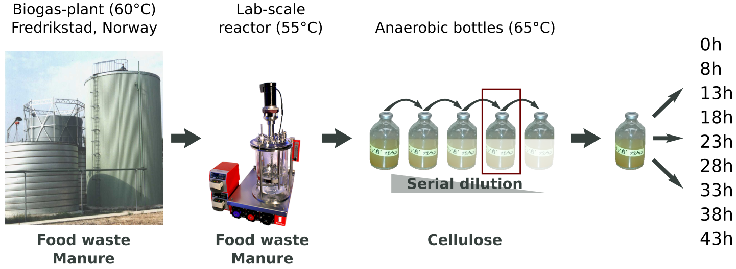
The sample studied in this work originated from a thermophilic biogas-plant operated on muncipal food waste and manure. After a round in a lab-scale reactor, we performed a serial dilution to extinction experiment to simplify and enrich the community for growth on cellulose (Norwegian Spruce).

Metagenomics:

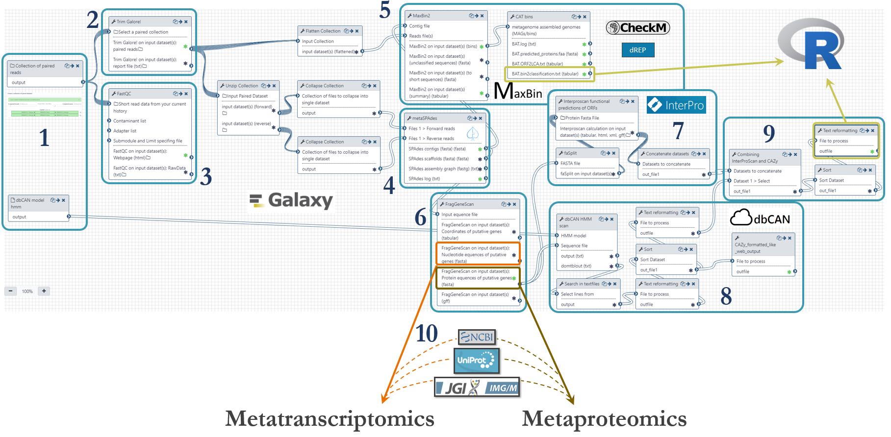
An Illumnia HiSeq 3000 platform was used for metagenomics shotgun sequencing of the microbial community. Samples were sequenced with paired ends (2 x 125 bp) on four lanes. These were the steps of the metagenomics analysis workflow, numbered according to the figure below:

1. Fastq-files were uploaded to Galaxy via ftp (~45Gb per file) and organized as a Collection of paired datasets. The Hidden Markov Model (HMM) for prediction of CAZymes was downloaded from http://bcb.unl.edu/dbCAN2/download/ and uploaded to Galaxy.
2. Trimming of reads were done with Trim Galore! with automatic detection of adapter sequences.
3. Quality control with FastQC to assess the overrepresentation of features (adapters/primers) and Phred threshold of 20.
4. To assemble metagenomic reads into contigs we used metaSPAdes with k-mer sizes of 21,33,55 and 77.
5. Binning of contigs was done based on an expectation-maximization algorithm using MaxBin2. We used a minimum contig length of 5000. Taxonomical placement was done with the Bin Annotation Tool, and each bin’s completeness, contamination and strain heterogeneity was checked using CheckM (currently not in Galaxy). We are also working on an implementation of dREP (that also include CheckM) for further validation of the bins. The abundance table provided by MaxBin2 were used to generate a cluster plot to visualize the bins (figure further down).
6. We predicted genes using the software FragGeneScan
7. The putative proteins from FragGeneScan were functionally annotated using InterProScan with the following databases: TIGERFAM, HAMAP, PfamA, Gene Ontology, EC and KEGG.
8. Prediction of CAZymes were done using the Hidden Markov Models from dbCAN and the software HMMER.
9. We then combined all the functional annotations from InterProScan and dbCAN into one file for downstream analysis using the Galaxy implementation of awk to generate a tabular with one protein per row and the different annotations in individual columns. This file was used as input of R-scripts to count the presence of specific enzymes in the metagenome (described further down).
10. The putative genes and proteins (fasta-files) from FragGeneScan can be manually augmented with strains from public repositories such as NCBI, UniProt or IMG.

The metagenomics workflow is shared publicly and can be found here

Metatranscriptomics:

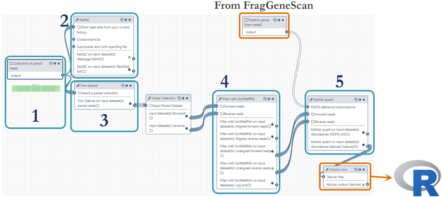
Samples were taken at different timepoints during the lifetime of the microbial community, as indicated in the figure above. For this analysis, we used the time points 13h, 23h and 38h. mRNA extraction was performed in triplicate and was sequenced with paired-end technology (2 x 125 bp) on one lane of an Illumnia HiSeq 3000 system. These were the steps of the metatranscriptomics analysis workflow, numbered according to the figure below:

1. Fastq-files were uploaded to Galaxy via ftp (~45Gb per file) and organized as a Collection of paired datasets.
2. Quality control with FastQC to assess the overrepresentation of features (adapters/primers)
3. Trimming was done using Trim Galore! with automatic detection of adapter sequences and Phred threshold of 20.
4. rRNA and tRNA were removed using the software SortMeRNA.
5. Quantification of mRNA was done with the pseudoaligment software Kallisto by mapping the transcripts to the putative genes predicted by FragGeneScan in the metagenomics workflow. The outputs from Kallisto, one per sample-pair, were joined in order to generate one single file for import to R.

The metatranscriptomics workflow is shared publicly and can be found here

Metaproteomics:

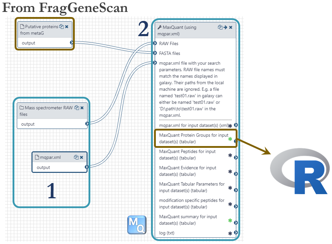
Samples for proteomics were taken for every timepoint as indicated in the dataset-figure above. For this analysis, we used the same time points as we used for metatranscriptomics, 13h, 23h and 38h. Each sample were separated into 16 fractions by SDS-PAGE, cut out and digested with trypsin before analyzed on a Q-Exactive (Thermo) mass spectrometer. These were the steps of the metaproteomics analysis workflow, numbered according to the figure below:

1. 144 mass spectrometer RAW files were uploaded to Galaxy using the web interface (~1Gb per file). A local Windows-installation of MaxQuant version 1.6.3.4 (NB: same version as on Galaxy!) was used to generate a configuration file (mqpar.xml) with all the necessary settings. This configuration file was then uploaded to Galaxy as used as input.
2. Identification and quantification of proteins were accomplished using the software MaxQuant by mapping MS/MS spectra to putative proteins predicted by FragGeneScan in the metagenomics workflow. The Protein Groups file was used as input in downstream R-scripts.

The metaproteomics workflow is shared publicly and can be found here

Integration of omics data using R:

For the following, a stand-alone version of RStudio can be used, or one can utilize the live RStudio which has direct access to the data residing in the Galaxy History.

The files needed to generate the following plots are:

• Abundance table from MaxBin2
• List of bins (contigs in FASTA-format)
• The combined annotation file from dbCAN and InterProScan
• The combined quantification file from Kallisto
• ProteinGroups.txt from MaxQuant

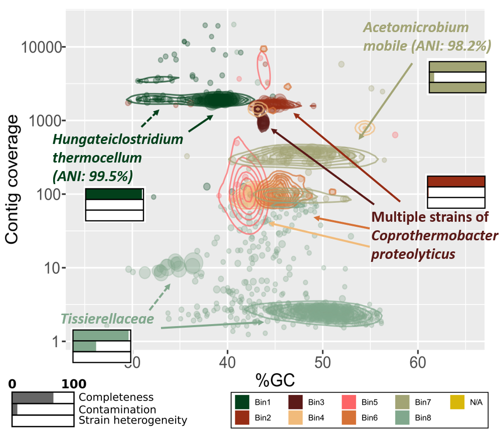
The first plot to consider is the phylogenetic binning of contigs. In our workflow the binning was accomplished using metagenomic reads and the assembled contigs from metaSPAdes. This produced two outputs of specific interest, an abundance file and a list of the bins. The latter is in FASTA format and one file per bin exist. Our script reads these files and generate a list of contigs with information about the contig abundance and which bin it belongs to. Then, we plot the contig's GC% vs. abundance using ggplot in R and color it by bin. A metagenome-assembled genome (MAG), or bin, typically has a well-clustered layout in this plot, which can be highlighted with the geom_density2d function.

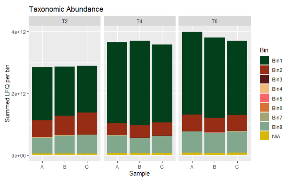
Taxonomic abundance plots can be calculated either from metaproteomics or metatranscriptomics data, using the summed abundances (not log2'ed!) of all mRNA/proteins per bin. Here we calculated the summed LFQ (label-free quantification) values reported by MaxQuant. The most abundant community member at all time points was Bin1, Hungateiclostridium thermocellum.

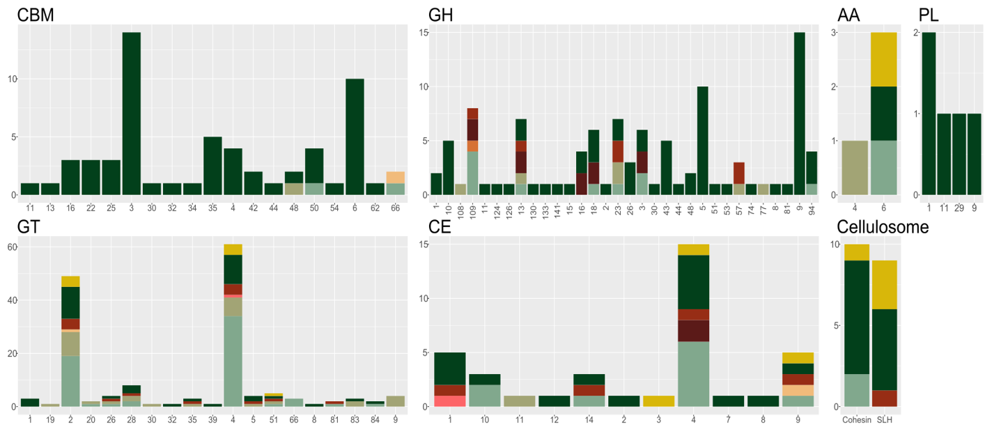
Further, we can generate an overview of all CAZymes in the microbial community. This can of course be made for any functional annotation, but here we are focussing on CAZymes. We use the annotation file from dbCAN and InterProScan and filter this for only CAZymes. Note that CAZymes are modular domains and enzymes can therefore harbour multiple CAZy domains; in our case this means that the CAZy column is semicolon-separated. In Tidyverse, there is a function to split multiple terms within one column into several rows, keeping all the other information, see separate_rows.

This overview plot suggests that Bin1 (Hungateiclostridium thermocellum) is the main polysaccharide hydrolyser, and further, that it utilizes cellulosomes, i.e. large enzyme complexes where many enzymes can degrade cellulose simulateously. The monomer, glucose, is used by the many suger fermenters present in the community.

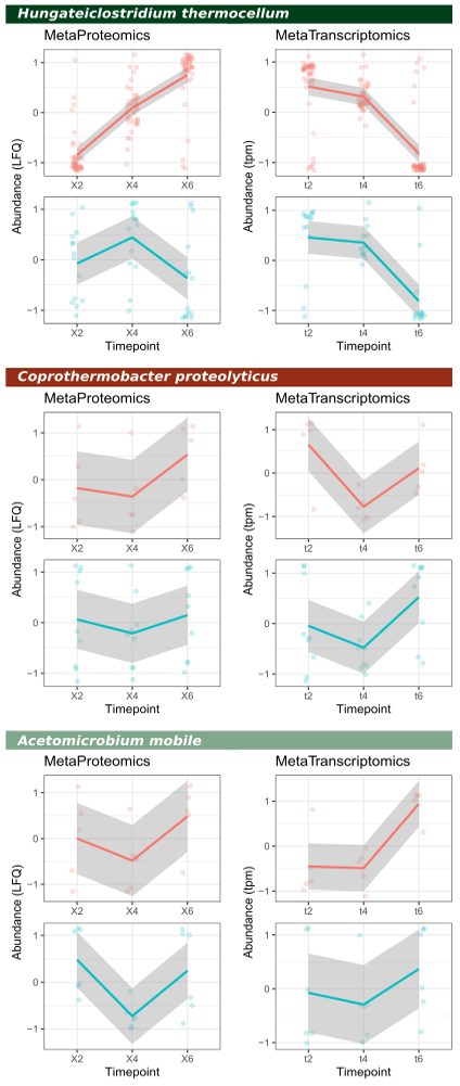
For this dataset we have two 'functional layers', mRNA and protein. We can therefore calculate quantification of individual enzymes, or for enzyme classes, or even at pathway-level by utilizing e.g. the EC-annotation available within the InterProScan annotation file. For this example, we have focussed on two enzyme classes, glycoside hydrolases and glycosyl transferases; these are colored red and blue in the below figure, respectively.
For this we need the ProteinGroups.txt file from MaxQuant, and the combined quantification file from Kallisto. We use the 'Majority protein IDs' (up to first semicolon) as geneID for metaproteomics and 'target_id' as geneID for metatranscriptomics. In Tidyverse, we can join the two tables based on these common identifiers by using the function full_join. As quantitative values we use LFQ (label-free quantification) for proteomics and tpm (transcript per million) for transcriptomics. Both values need to be log2-transformed. Note that ggplot (and Tidyverse in general) does not work with tables with quantification values in different columns. We therefore need to 'melt' the table to generate a one-column value representation. This can be accomplished using the pivot_longer function. Then finally, to visualize the trends in quantification over time, we apply a z-score normalization per protein/transcript, independently for each omics.

Note that the trends in quantification at enzyme-class level is by and large similar; however, for some classes there are differences. This can be linked to the half-life of molecules, which is just a few minutes for mRNA while up to hours for proteins.

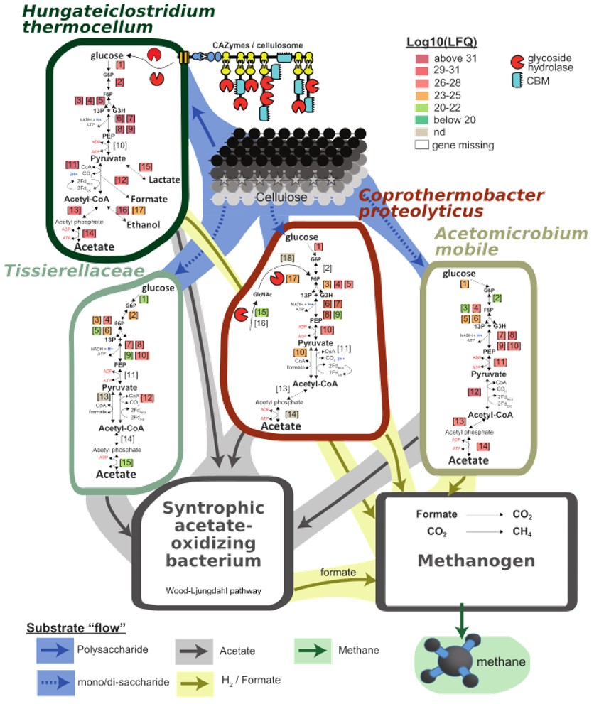
The last plot cannot be generated using a R-script, unfortunately, but rather require your ulitmate Illustrator/Inkscape skills. This is a plot of the inferred carbon flow within the microbial community, based on the plots and data above. The metagenomics provided us with MAGs present in our community, and the functional annotaion allowed us to predict what each of them were capable of doing. Metatranscriptomics and metaproteomics provided us with information about what they were actually doing, and who was doing what. Additional community metadata, such as gas analysis, reveiled that the final product was methane. We can then draw a graph of anaerobic degradation, starting with cellulose being converted in glucose, that is converted further to acetate. A syntrophic acetate oxidizing bacterium and a methanogetn (both not identified in this proof-of-principle Galaxy implementation, but in the full dataset) converts acetate further to formate, CO2, H2 and methane.

Here we have drawn the relevant pathways and decorated them with metaproteomics LFQ-values (from the full dataset). This suggests that cellulose is primarily degraded by Hungateiclostridium thermocellum while the cellulose monomer, glucose, is fermented to acetate by Coprothermobacter proteolyticus, Acetomicrobium mobile and Tissierellaceae.

Acknowledgements:

This work was funded by the Norwegian Centennial Chair Programme.

This study has been described in its entirey here:

• Kunath BJ, Delogu F, et. al. From proteins to polysaccharides: lifestyle and genetic evolution of Coprothermobacter proteolyticus. ISME J. 2019 Mar; 13(3):603-617
• Delogu F, Kunath BJ, et. Al. Integration of absolute multi-omics reveals translational and metabolic interplay in mixed-kingdom microbiomes. bioRxiv.

Contributors:

Norwegian University of Life Sciences:

• Francesco Delogu
• Benoit Kunath
• Phil Pope

University of Minnesota:

• Praveen Kumar
• Subina Mehta
• James E. Johnson
• Pratik Jagtap
• Timothy J. Griffin

University of Freiburg:

• Bjoern Gruning