Galaxy 101 - What is Galaxy?

Before diving into a practical exercise let us introduce several fundamental concepts about Galaxy.

What is Galaxy Project?

According to wikipedia "a galaxy is a gravitationally bound system of stars, stellar remnants, interstellar gas, dust, and dark matter". In other words it is a system composed of multiple components. Likewise the Galaxy Project also consists of multiple components including:

• The Galaxy Software Framework
• The Public Galaxy Service

The Galaxy software framework

Galaxy software framework is an open-source application (distributed under the permissive Academic Free License). Its goal is to develop and maintain a system that enables researchers without informatics expertise to perform computational analyses through the web. A user interacts with Galaxy through the web by uploading and analyzing the data. Galaxy interacts with underlying computational infrastructure (servers that run the analyses and disks that store the data) without exposing it to the user.

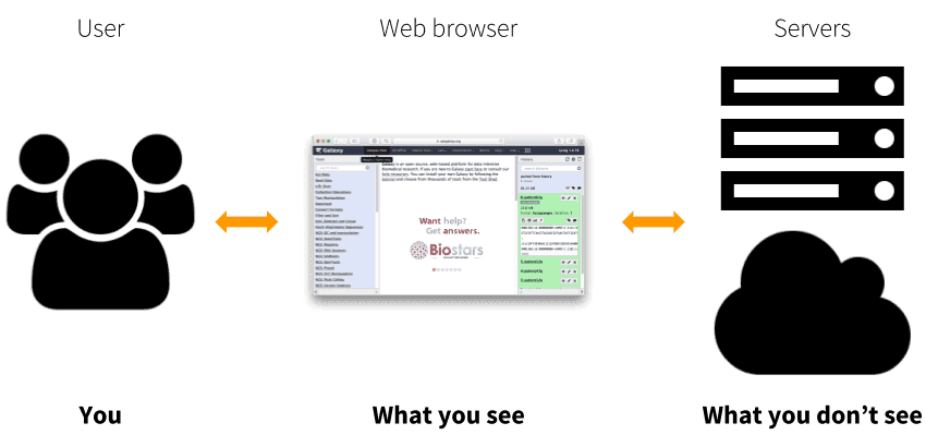Figure 1. Galaxy is a web application that allows processing of large datasets using powerful infrastructure that the user never sees or directly interacts with. This infrastructure can be a conventional cluster, a cloud, or any combination of the two.

The Public Galaxy Service

The main Galaxy instance at https://usegalaxy.org is an installation of the Galaxy software combined with many common tools and data; this site has been available since 2007 for anyone to analyze their data free of charge. The site provides substantial CPU and disk space, making it possible to analyze large datasets. The site supports thousands of users and hundreds of thousands of jobs per month (see https://bit.ly/gxystats). It is sustained by TACC hardware using allocation generously provided by the CyVerse project.

In addition to the main Galaxy instance there numerous other sites running Galaxy software framework featuring different sets of tools and alternative interfaces. These can be explored at out public servers page.

What is the goal of this tutorial?

In this tutorial we will introduce you to bare basics of Galaxy:

• Getting data from external databases such as UCSC
• Performing simple data manipulation
• Understanding Galaxy's History system
• Creating and running a workflow (Part 2)

The research question

In this example we will use Galaxy to answer the following question:

Before you begin: Organizing your windows and setting up Galaxy account

To make this demonstration smooth we would recommend setting up your workspace as described below:

Getting your display sorted out

To get the most of this tutorial open two browser windows. The first is the one you already have (this page). To open the other, right click this link and choose "Open in a New Window" (or something similar depending on your operating system and browser):

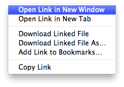Figure 2. Open a new window by right clicking this link.

Then organize your windows as something like this (depending on the size of your monitor you may or may not be able to organize things this way, but you get the idea):

Figure 3. Two screens side by side will make it easy for you to follow this tutorial.

Setting up Galaxy account

Go to the "Login or Register" link at the top of Galaxy interface and choose "Register" (unless of course you already have an account):

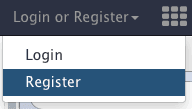Figure 4. To create a user account use "Login or Register" link on top of Galaxy interface.

Then enter your information and you're in!

Getting data

Our research problem calls for using existing annotation of human genome (we will use exons and SNPs that are already annotated across the genome sequence). So to answer our question we need to compare coordinates of exons and SNPs against each other. One of the most frequently used repositories of genome annotation data is maintained by the Genome Informatics Group at the University of California at Santa Cruz.

Getting coding exons

First thing we will do is to obtain exon coordinate data from UCSC by clicking Get Data → UCSC Main:

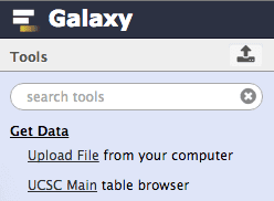Figure 5. Expand "Get Data" category and click on "UCSC Main".

You will see UCSC Table Browser interface appearing in your browser window:

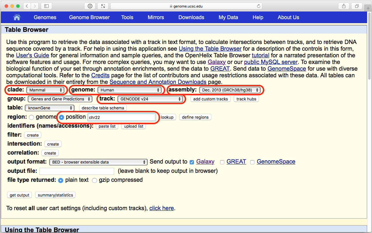Figure 6. The UCSC Table Browser interface. Verify that parameters highlighted in red are set as shown here.

Make sure that your settings are exactly the same as shown Fig. 6 (in particular, position should be set to "chr22", output format should be set to "BED - browser extensible data", and "Galaxy" should be checked within the Send output to option). Click get output and you will see the next screen:

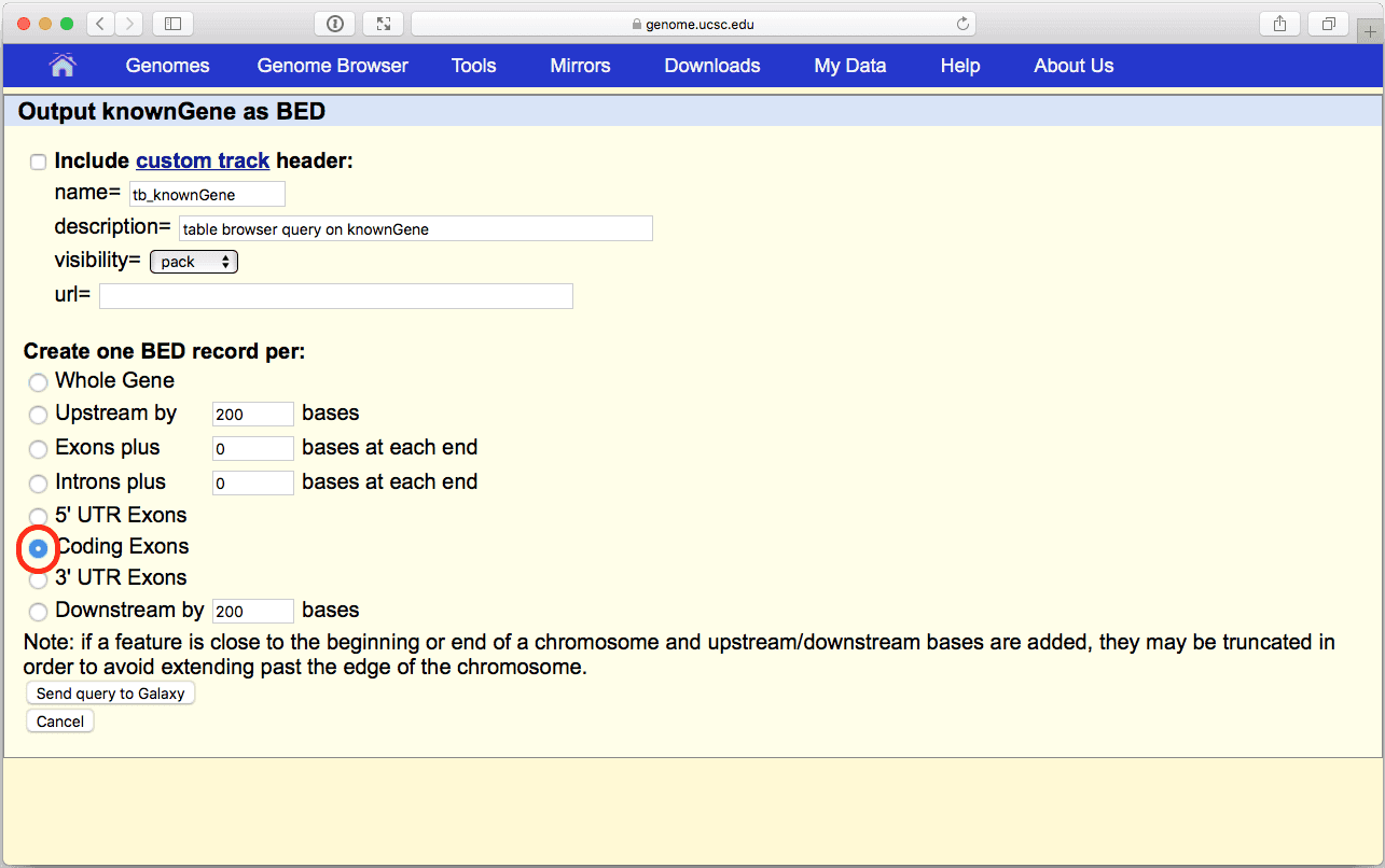Figure 7. BED output screen of the UCSC Table Browser interface. Here make sure you select "Coding Exons" radio button.

Make sure Create one BED record per: is set to "Coding Exons" and click Send Query to Galaxy button. After this you will see your first History Item in Galaxy's right pane. It will go through gray (preparing) and yellow (running) states to become green:

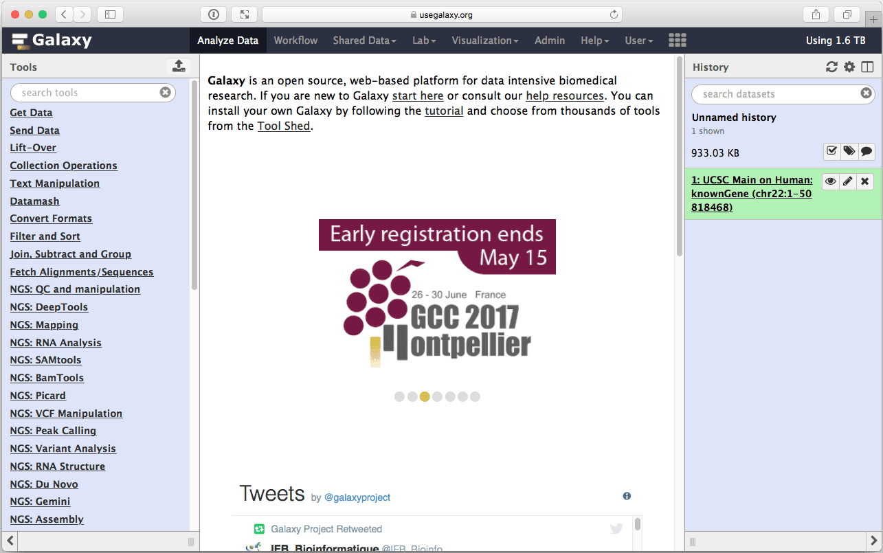Figure 8. The first dataset in the history (right pane) contains data about location of coding exons on chromosome 22.

Getting SNPs

Now is the time to obtain SNP data (SNPs are single nucleotide polymorphisms). This is done almost exactly the same way except now we will need to make a different set of choices within the UCSC Table Browser interface. First thing we will do is to again click on Get Data → UCSC Main:

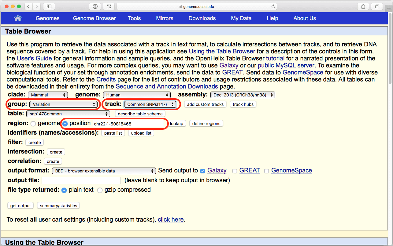Figure 9. The UCSC Table Browser interface. Verify that parameters highlighted in red are set at shown here.

click "get output" and you should see this:

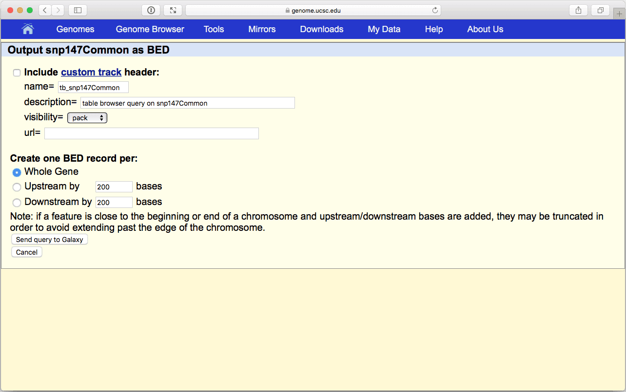Figure 10. BED output screen of the UCSC Table Browser interface. Here you do not need to modify any settings.

where you do not need to change anything (make sure that Whole Gene is selected ("Whole Gene" here really means "Whole Feature") and click Send Query to Galaxy button. You will get your second item in the history:

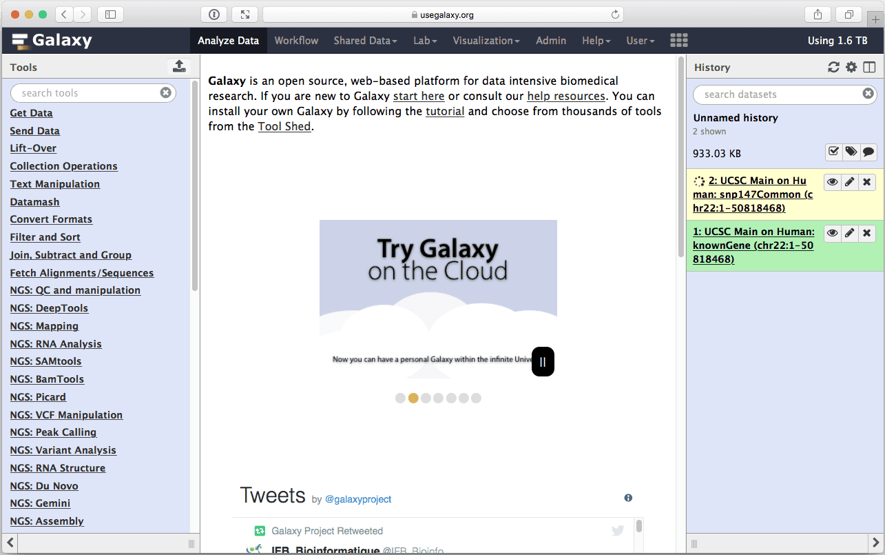Figure 11. History with two datasets.

Tidying up

Now we will rename the two history items to "Exons" and "SNPs" by clicking on the Pencil icon adjacent to each item. You will see middle pane of the interface changing. There (in the middle pane) you will have the opportunity to rename datasets. After changing the name scroll down and click Save. Also we will rename history to "my example" (or whatever you want) by clicking on Unnamed history so everything looks like this:

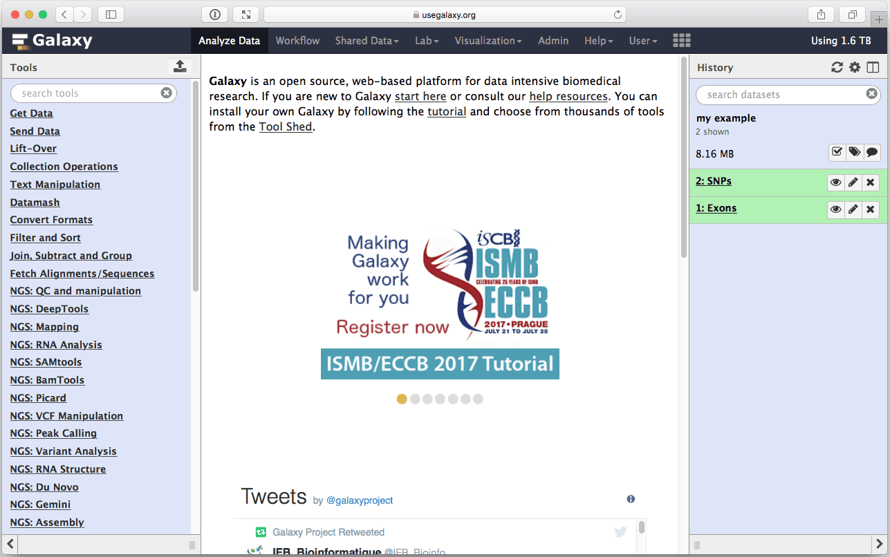Figure 12. History after datasets were renamed.

Finding Exons with the highest number of SNPs

Joining exons with SNPs

Let's remind ourselves that our objective was to find which exon contains the most SNPs. This first step in answering this question will be joining exons with SNPs (a fancy word for finding exons and SNPs that overlap side by side). This is done using Operate on Genomics Intervals → Join tool:

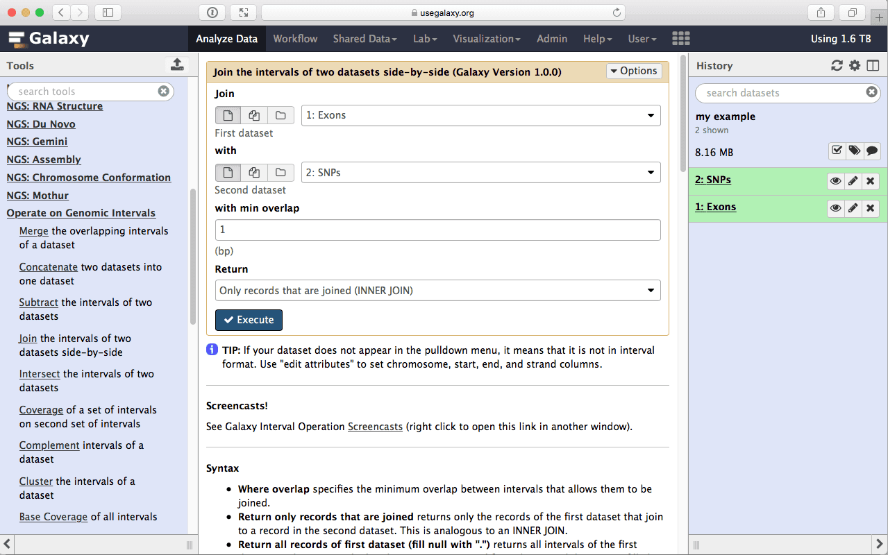Figure 13. To join exons with SNPs select "Exons" as the first dataset and "SNPs" as the second.

make sure your Exons are first and SNPs are second and click Execute. Note that you can drag and drop datasets from History into tool interface input selectors:

Figure 13A. You can drag and drop datasets!

You will get the third history item:

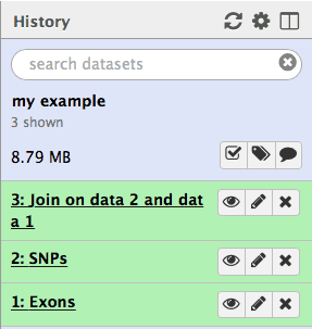Figure 14. The third history item is the result of joining of the first (Exons) with the second (SNPs). Each subsequent analysis operation will add additional items to the growing history.

Counting the number of SNPs per exon

Look at the data obtained from the join operation above (you can do it by clicking the eye icon adjacent to the dataset). Below is a subsample of rows from the joined datasets (you may need to scroll sideways to see the entire length of the rows below):

chr22 15710867 15711034 uc062bej.1_cds_9_0_chr22_15710868_f  0 + chr22 15710880 15710881 rs568292779 0 -
chr22 15710867 15711034 uc062bej.1_cds_9_0_chr22_15710868_f  0 + chr22 15710947 15710948 rs544633418 0 -
chr22 15710867 15711034 uc062bej.1_cds_9_0_chr22_15710868_f  0 + chr22 15710906 15710907 rs548691624 0 -
chr22 15710867 15711034 uc062bej.1_cds_9_0_chr22_15710868_f  0 + chr22 15710920 15710921 rs530488686 0 -
chr22 15710867 15711034 uc062bej.1_cds_9_0_chr22_15710868_f  0 + chr22 15710932 15710933 rs563306354 0 -
chr22 15710867 15711034 uc062bej.1_cds_9_0_chr22_15710868_f  0 + chr22 15711019 15711020 rs559431407 0 -
chr22 15710867 15711034 uc062bej.1_cds_9_0_chr22_15710868_f  0 + chr22 15710949 15710950 rs532940301 0 -

                                                      ....

chr22 15719659 15719777 uc062bej.1_cds_10_0_chr22_15719660_f 0 + chr22 15719668 15719669 rs200891952 0 -
chr22 15719659 15719777 uc062bej.1_cds_10_0_chr22_15719660_f 0 + chr22 15719751 15719752 rs556077431 0 -

Look at the rows. They all correspond to the same exon (id = uc062bej.1_cds_9_0_chr22_15710868_f) that overlaps seven distinct SNPs (ids: rs568292779, rs544633418, rs548691624, rs530488686, rs563306354, rs559431407, rs532940301). In other words this means that this exon contains seven SNPs. Since our ultimate goal is to count the number of SNPs per exon we can simply do this by counting how many times an exon's id appears in this dataset. This can be easily done with the Join, Subtract, and Group → Group tool:

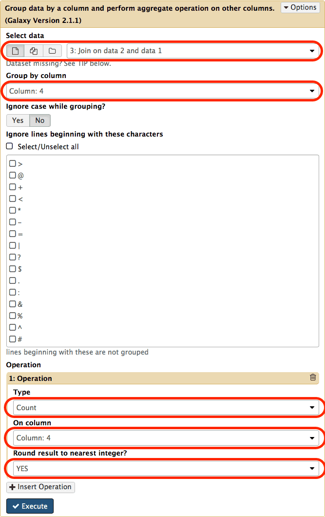Figure 15. Grouping tool interface. Set parameters as highlighted with red outlines. To reveal operation interface at the bottom click on Insert Operation button.

click Execute. Your history will look like this:

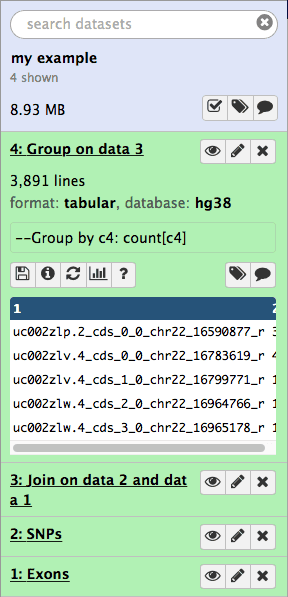Figure 16. Results of grouping operation appear as the fourth item in the history.

if you look at the above image you will see that the result of grouping (dataset #4) contains two columns. This first contains the exon name while the second shows the number of times this name has been repeated in dataset #3:

uc002zlp.2_cds_0_0_chr22_16590877_r    3
uc002zlv.4_cds_0_0_chr22_16783619_r    4
uc002zlv.4_cds_1_0_chr22_16799771_r    1
uc002zlw.4_cds_2_0_chr22_16964766_r    1

the number in the second column is effectively the number of SNPs that exon contains.

Sorting exons by SNP count

To see which exon has the highest number of SNPs we can simply sort the dataset #4 on the second column in descending order. This is done with Filter and Sort → Sort:

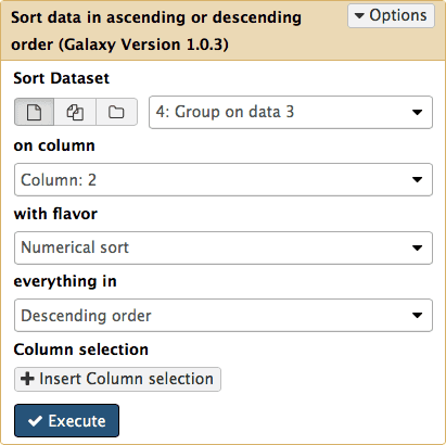Figure 17. Sorting results by SNP count in descending order.

This will generate the fifth history item:

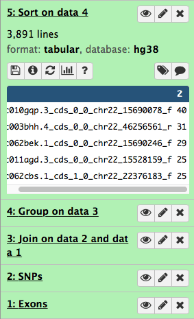Figure 18. Sorting generates the fifth item in the history.

and you can now see that the highest number of SNPs per exon is 40.

Selecting top five

Now let's select top five exons with the highest number of SNPs. For this we will use Text Manipulation → Select First tool:

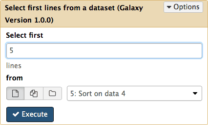Figure 19. Selecting the first five lines.

Clicking Execute will produce the sixth history item that will contain just five lines:

uc010gqp.3_cds_0_0_chr22_15690078_f   40
uc003bhh.4_cds_0_0_chr22_46256561_r   31
uc062bek.1_cds_0_0_chr22_15690246_f   29
uc011agd.3_cds_0_0_chr22_15528159_f   25
uc062cbs.1_cds_1_0_chr22_22376183_f   25

Recovering exon info and displaying data in genome browsers

Now we know that in this dataset the five top exons contain between 25 and 40 SNPs. But what else can we learn about these? To know more we need to get back the positional information (coordinates) of these exons. This information was lost at the grouping step and now all we have is just two columns with IDs and counts. To get coordinates back we will match the names of exons in dataset #6 (column 1) against names of the exons in the original dataset #1 (column 4). This can be done with Join, Subtract and Group → Join tool (note the settings of the tool in the middle pane):

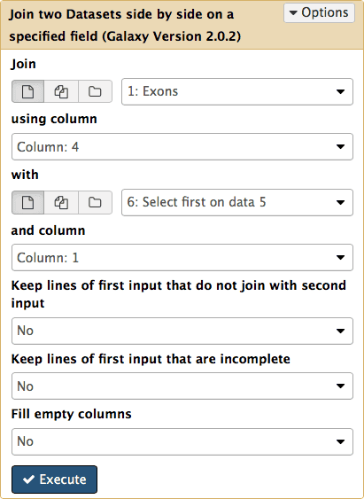Figure 20. Joining the first history dataset (Exons) with dataset #6 (sorting results) will retrieve those records from dataset #1 which share IDs with dataset #6.

this adds the seventh dataset to the history in which lines from datasets #1 and #6 are joined line-by-line:

chr22 15528158 15529139 uc011agd.3_cds_0_0_chr22_15528159_f 0 + uc011agd.3_cds_0_0_chr22_15528159_f 25
chr22 15690077 15690709 uc010gqp.3_cds_0_0_chr22_15690078_f 0 + uc010gqp.3_cds_0_0_chr22_15690078_f 40
chr22 15690245 15690709 uc062bek.1_cds_0_0_chr22_15690246_f 0 + uc062bek.1_cds_0_0_chr22_15690246_f 29
chr22 22376182 22376505 uc062cbs.1_cds_1_0_chr22_22376183_f 0 + uc062cbs.1_cds_1_0_chr22_22376183_f 25
chr22 46256560 46263322 uc003bhh.4_cds_0_0_chr22_46256561_r 0 - uc003bhh.4_cds_0_0_chr22_46256561_r 31

Visualizing results

The best way to learn about these exons is to look at their genomic surrounding. There is really no better way to do this than using genome browsers. Because this analysis was performed on "standard" human genome (hg38 in this case), you have two choices - UCSC Genome Browser and IGV.

However, before we begin we need to prepare data. The problem is that browsers expect data in certain format. In particular the UCSC Genome Browser "plays well" with datasets in BED format. To convert the data shown above into BED format we need:

1. replace data in column 5 with data from the last column
2. remove duplicate IDs (retain only column 4 and remove column 7)

The first step will set score columns of BED format to the number of SNPs and the second will reduce out data to six columns required by BED specification (BED6). Both of these steps can be performed with a single tool Text manipulation → Cut tool (the second one in the list, not the first one) by cutting out columns 1, 2, 3, 4, 8, and 6:

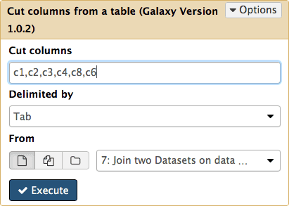Figure 21. Cutting columns c1,c2,c3,c4,c8,c6 from dataset #7. Here c is short for "column". Column numbers start with 1.

The resulting dataset looks like this:

chr22 15528158 15529139 uc011agd.3_cds_0_0_chr22_15528159_f 25 +
chr22 15690077 15690709 uc010gqp.3_cds_0_0_chr22_15690078_f 40 +
chr22 15690245 15690709 uc062bek.1_cds_0_0_chr22_15690246_f 29 +
chr22 22376182 22376505 uc062cbs.1_cds_1_0_chr22_22376183_f 25 +
chr22 46256560 46263322 uc003bhh.4_cds_0_0_chr22_46256561_r 31 -

This is exactly as BED6 should look like. However, Galaxy does not know that this is BED6, so we need to tell it that. To do this click on pencil icon adjacent to the latest history dataset and click on "Datatype" tab:

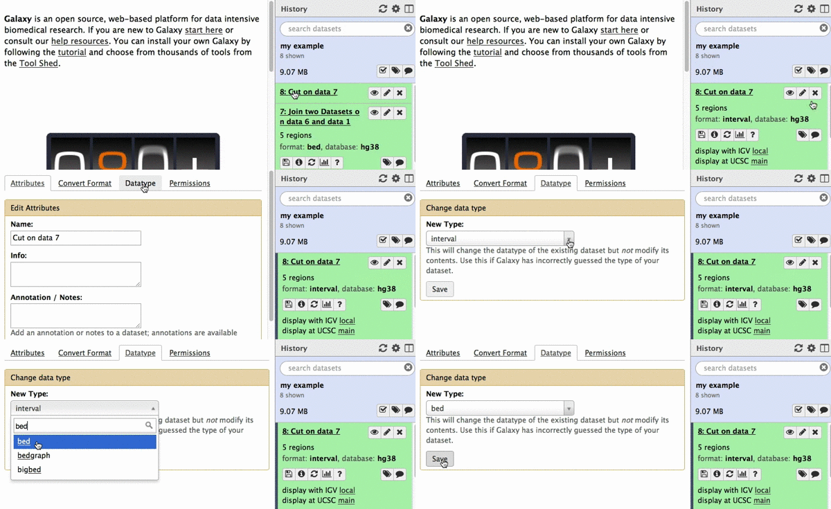Figure 22. Changing datatype to BED.

After changing the datatype the history item will reveal UCSC Browser link:

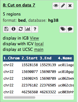Figure 23. After changing format to BED UCSC link becomes visible.

Let's click in this "display at UCSC main" link. This open a new tab within your web browser:

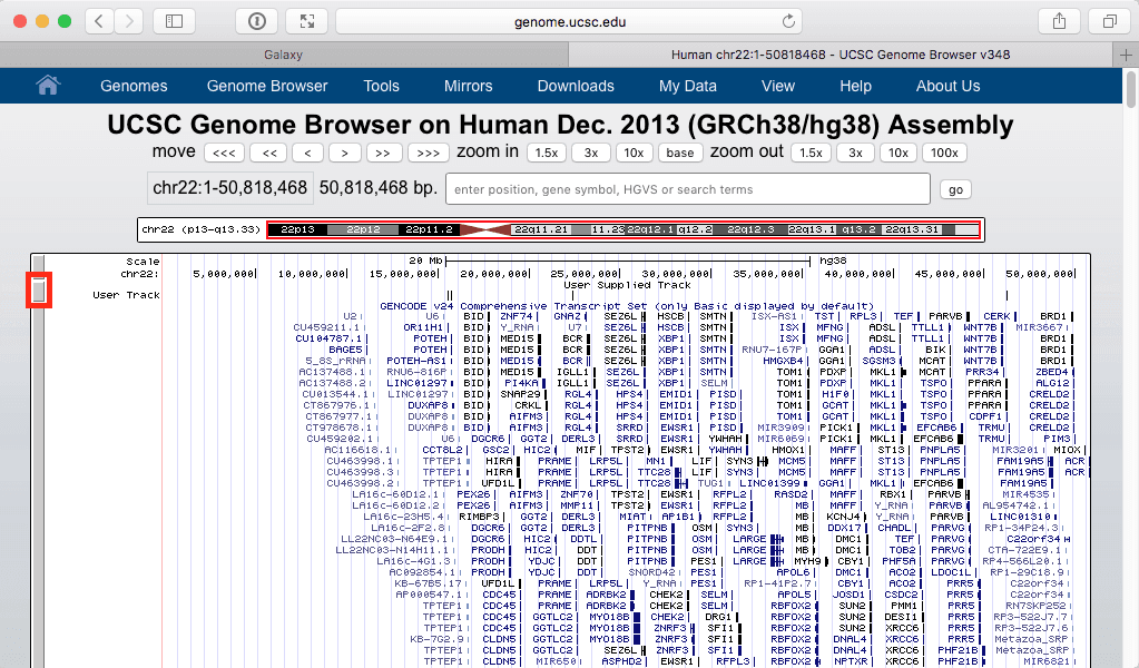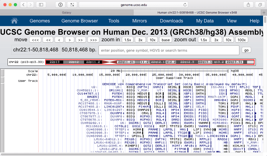
Figure 24. UCSC Genome browser displaying dataset #8 as a "User Track". Make sure that you can see the entire chromosome by using zoom settings of the browser.

The above figure shows out five exons widely spread out across chromosome 22. But which one contains the highest number of SNPs? Since we know that the highest number is 40 we can filter visible regions of the "User track" to show only those that have number 40 in their score field (see Fig. 21). To do this click on a browser area highlighted with red rectangle in Fig. 24 above:

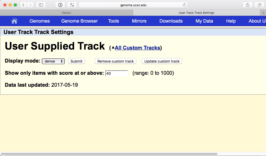Figure 25. Restricting visible regions to these with the score 40 of higher. Click "Submit" to see the effect of this filtering.

Filtering shows only one "User track" item on the browser:

Zooming in produces the following:
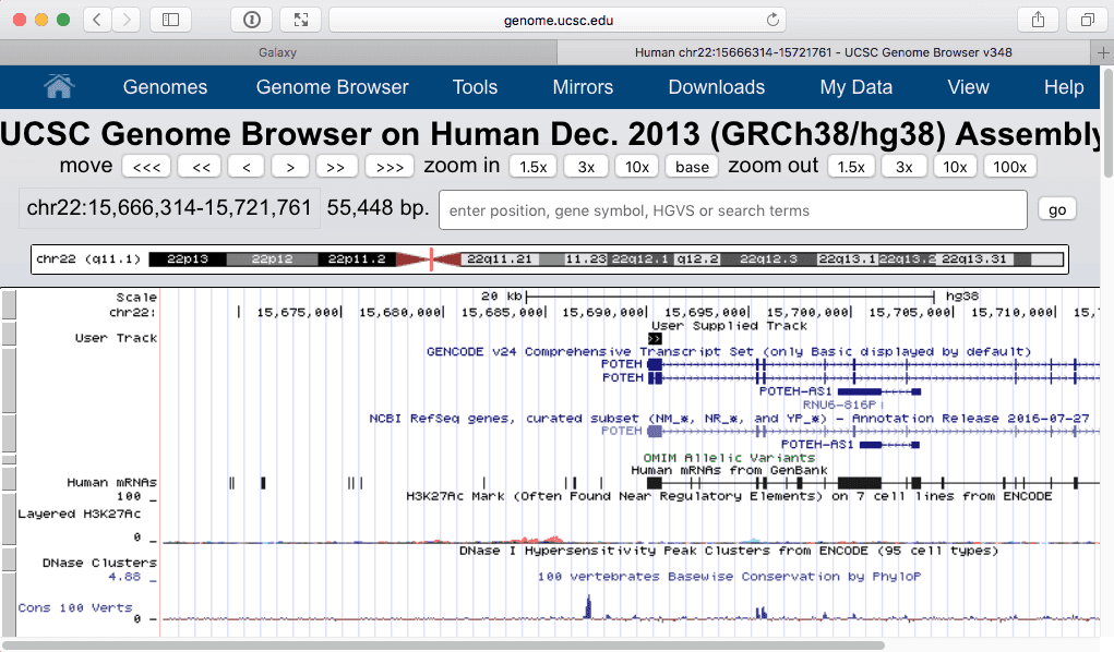Figure 26. The exon with the highest number of SNPs. Zooming in (lower part) shows that this is the first exons of POTEH gene.

Recap

In this tutorial we started with coordinates of exons and SNPs, found overlap between two datasets and narrowed it down to 5 exons containing the highest number of SNPs:

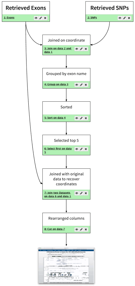Figure 27. Analysis outline. This looks like a workflow, doesn't it?

Creating and editing a workflow

You can see the an outline shown in Fig. 27 looks like a workflow. This is not coincidental - let's try to make a workflow from an analysis we just performed.

Extracting a workflow

Lets take a look at the history datasets generated during the analysis described above:

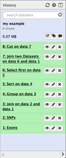Figure 28. History provides a complete record of the analysis. It can be converted into a workflow.

You can see that this history contains all steps of our analysis. So by building this history we have actually created a complete record of our analysis with Galaxy preserving all parameter settings applied at every step. Wouldn't it be nice to just convert this history into a workflow that we'll be able to execute again and again? This can be done by clicking on the cog icon and selecting Extract Workflow option:

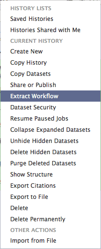Figure 29. History menu has an option for creating a workflow directly from history.

The center pane will change as shown below and you will be able to choose which steps to include/exclude and how to name the newly created workflow. In this case I named it g101:

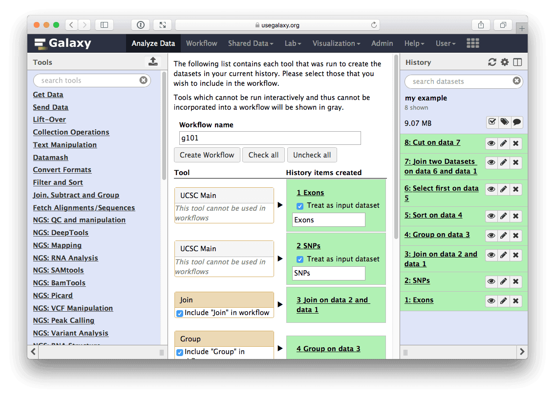Figure 30. Creating workflow from history. Here you can choose which steps should be included into workflow (in this case we include all) and name the workflow.

Once you click Create Workflow you will get the following message: "Workflow 'g101' created from current history. You can edit or run the workflow".

Opening workflow editor

Let's click edit (if you click something else and the message in the center page disappears, you can always access all your workflows including the one you just created using the Workflow link on top of Galaxy interface). This will open Galaxy's workflow editor. It will allow you to examine and change settings of this workflow as shown below. Note that the box corresponding to the Cut tool is selected (highlighted with the blueish border) and you can see parameters of this tool on the right pane. This is how you can view and change parameters of all tools involved in the workflow:

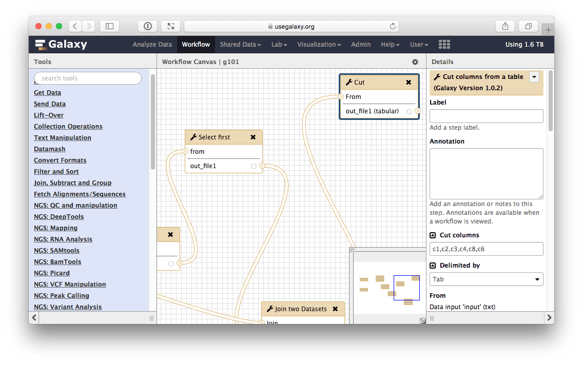Figure 31. Workflow editor can be used to modify all aspects of the workflow. Here cut tool is in focus and in the right pane of the interface you can see its settings. They are exactly as we set them when using this tool before (see Fig. 21).

The following image shows the workflow in its entirely. You can see that is exactly as was shown in Fig. 27 (well ... it has different shape but topologically it is the same).

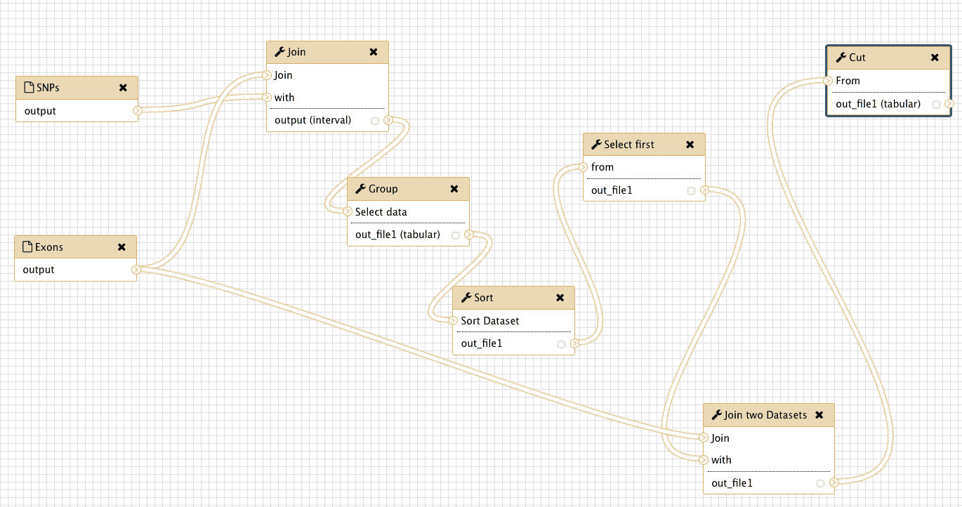Figure 32. Complete view of the workflow we have just created. You can see that it is exactly the same as in the theoretical outline shown in Fig. 27.

Hiding intermediate steps

When workflow is executed one is usually interested in the final product and not in the intermediate steps. These steps can be hidden by mousing over a small asterisk in the lower right corner of every tool:

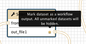Figure 33. Intermediate steps can be hidden by clicking on the asterisk within workflow elements.

Yet there is a catch. In a newly created workflow all steps are hidden by default and the default behavior of Galaxy is that if all steps of a given workflow are hidden, then nothing gets hidden in the history. This may be counterintuitive, but this is done to decrease the amount of clicking if you do want to hide some steps. So in our case if we want to hide all intermediate steps with the exception of the last one we will click that asterisk in last step of the workflow:

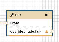Figure 34. Clicking an asterisk of the last element will make sure that a history element corresponding to this workflow step will be shown in the history minimizing clutter.

Once you do this the representation of the workflow in the bottom right corner of the editor will change with the last step becoming orange. This means that this is the only step, which will generate a dataset visible in the history:

Figure 35. An overview of the workflow in the bottom right corner of the editor shows which steps will produce visible history datasets. They are shown in orange.

Renaming inputs

Right now inputs are named after datasets that were in history from which this workflow was created. Let's give them more genetic names, so the workflow can be reused for other types of genome annotation data:

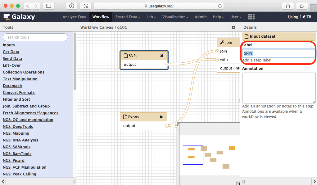Figure 36. To rename an input click on it and edit its name within the highlighted box.

Here we will simply rename input called "Exons" into "Feature 1" and the one called "SNPs" into "Feature 2":

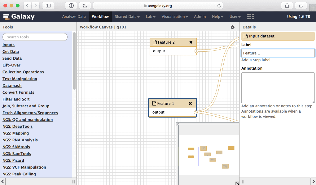Figure 37. Giving inputs genetic names.

Renaming outputs

Finally let's rename the workflow's output. For this:

• click on the last dataset (Cut)
• scroll down the rightmost pane and click on
• Type Top Exons in the Rename dataset text box:

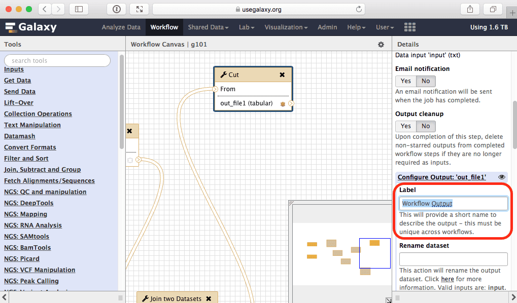Figure 38. Renaming workflow output.

Setting parameters "at runtime"

What we are trying to do here is do design a generic workflow. This means that from time to time you will need to change parameters within this workflow. For instance, in this tutorial we were selecting 5 exons containing the highest number of SNPs. But what if you need to select 10? Thus it makes sense to leave these types of parameters adjustable. Here is how to do this. First, select a tool in which you want to set parameters at runtime (Select first in this case):

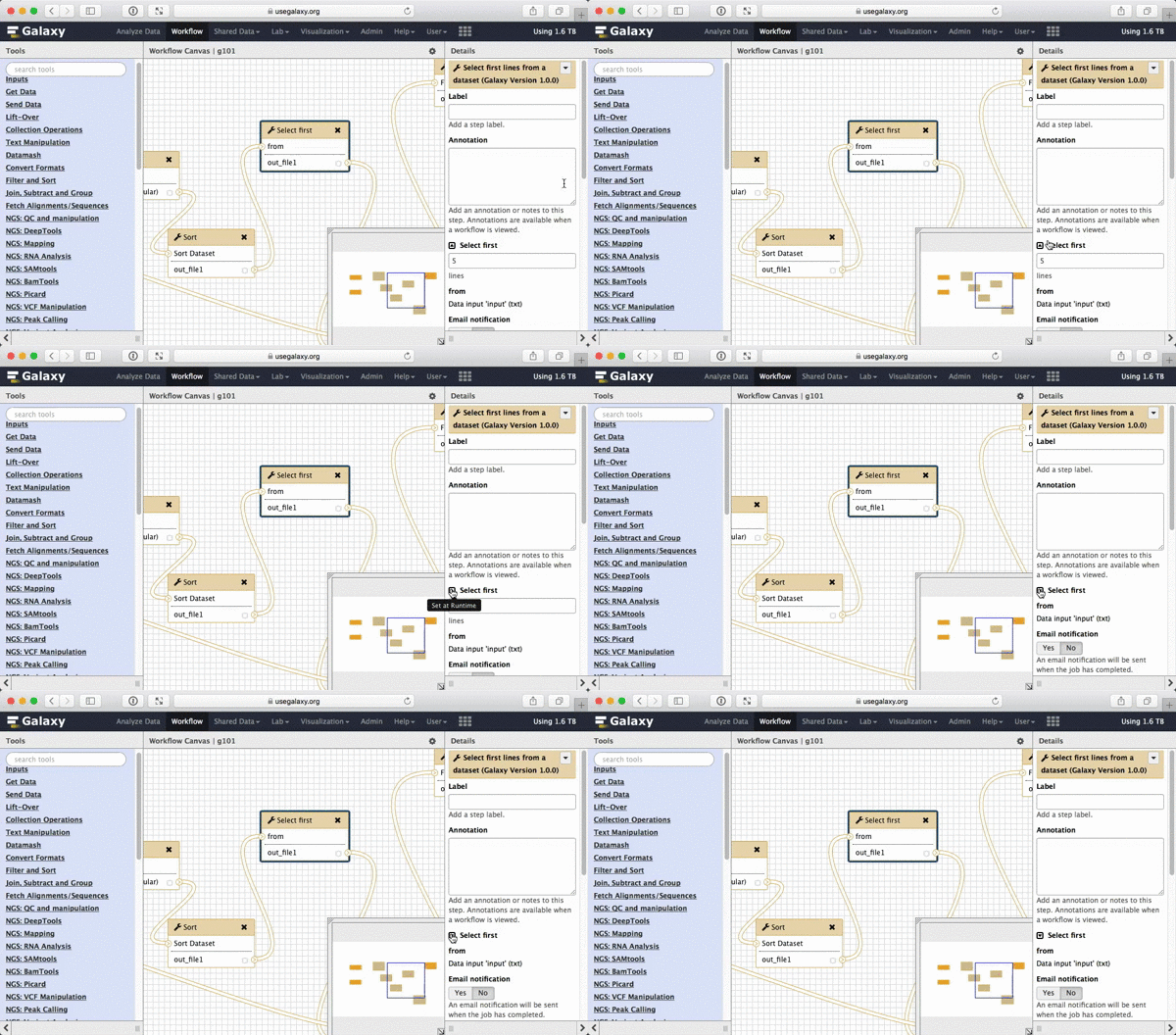Figure 39. To make a tool parameter settable at runtime simply click the icon.

Save! It is important...

Now let's save the changes we've made by clicking cog and selecting Save:

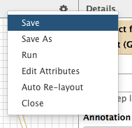Figure 40. Saving the workflow.

Run workflow on whole genome data

Now that we have a workflow, let's do something grand like, for example, finding exons with the highest number of repetitive elements across the entire human genome.

Get back in the Analysis mode

Curently the Galaxy interface is in the Workflow mode. To get back to the Analysis simply click "Analyze Data" link in the top of Galaxy interface.

Copy exon dataset to a new history

Since we already have exons in the history let's simply copy them into a new history. To do this click the cog icon and select "Copy Datasets":

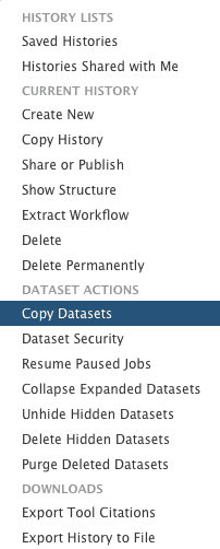Figure 41. Copying datasets starts will invoking "Copy Datasets" option within the history menu.

A new interface will appear in the middle pane. The following animated GIF shows next steps:

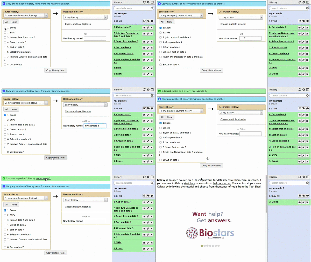Figure 42. To copy datasets select those you want to copy (just one in this case), give a name to the new history you want this dataset needs to be copied to ("my example 2"), click "Copy History Items". A green message "1 dataset copied to 1 history "my example 2" will appear. The name of the history in this message will be shown as a click-able link. Click on it and Galaxy will take you to a new history with only one dataset.

Get Repeats

Now let's retrieve coordinates of repetitive elements from the UCSC Table Browser. Use Get Data → UCSC Main:

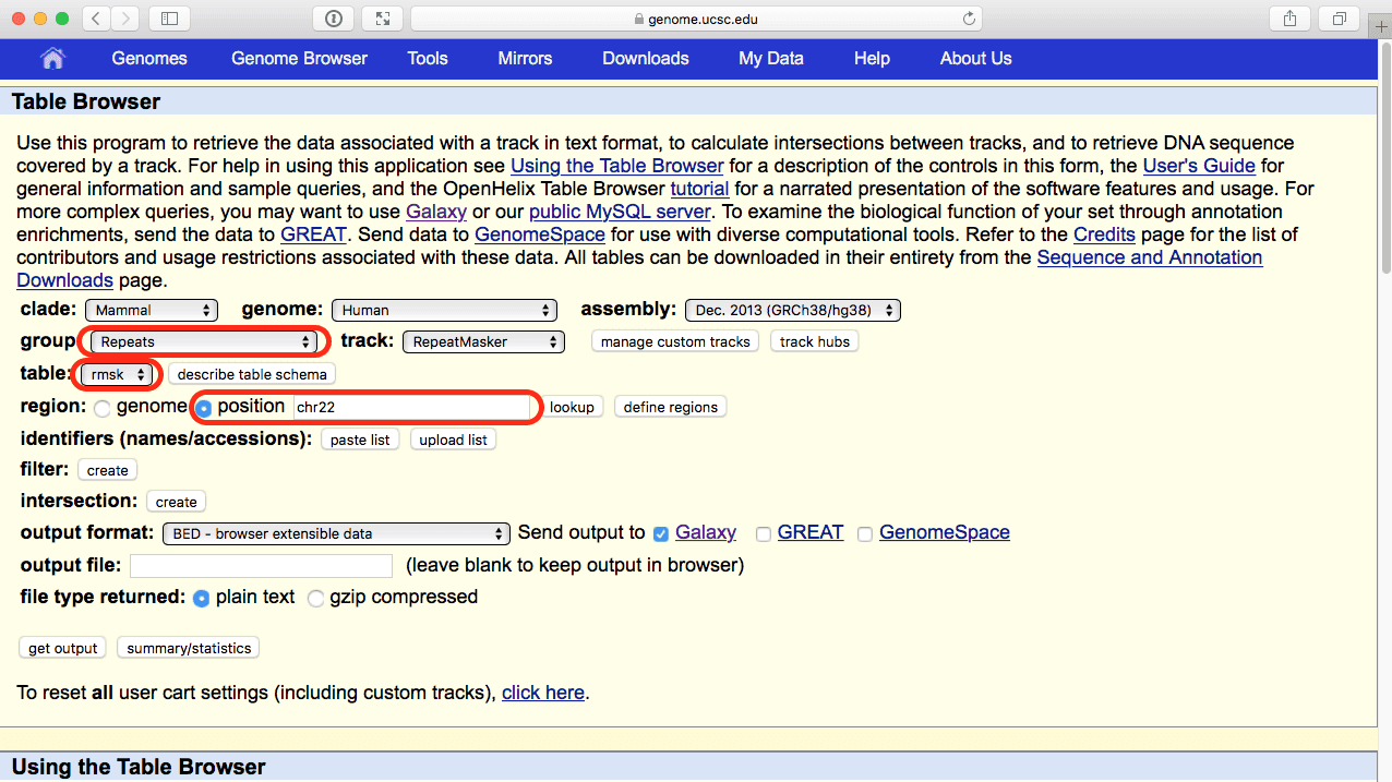Figure 43. Selecting repetitive elements annotated by RepeatMasker from the UCSC Table Browser. Note parameter selection highlighted with red outlines.

Click get output and you will get the next page (if it looks different from the image below, go back and make sure output format is set to BED - browser extensible format):

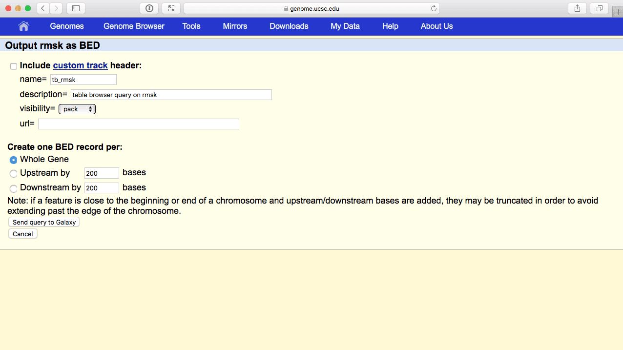Figure 44. BED output screen of the UCSC Table Browser. You do not need to modify anything here. Just make sure Whole gene is selected and click Send Query to Galaxy.

Finally, rename history item containing repetitive elements as "Repeats" (e.g., see Fig. 12).

Start the Workflow

At this point you will have two items in your history - one with exons and one with repeats. These datasets are large (especially repeats) and it will take some time for them to become green. Luckily you do not have to wait as Galaxy will automatically start jobs once uploads have ended. So nothing stops us from starting the workflow we have created. First, click on the Workflow link at the top of Galaxy interface, mouse over g101, click, and select Run. Center pane will change to allow you launching the workflow. Select appropriate datasets for Repeats and Exon inputs as shown below. Now scroll to Step 6 and will see that we can set up Select first parameter at Runtime (meaning Now!). So lets put 2 in there (or anything else you want) and scroll further down to click to see this:

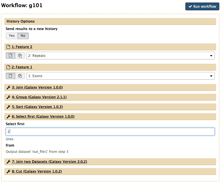Figure 45. Workflow launch interface. Note that "Exons" are selected as Feature 1 and "Repeats" as Feature 2. The number of lines in the Select first tool is set to "2".

Once workflow has started you will initially be able to see all its steps. Note that you are joining all exons with all repeats, so naturally this will take some time:

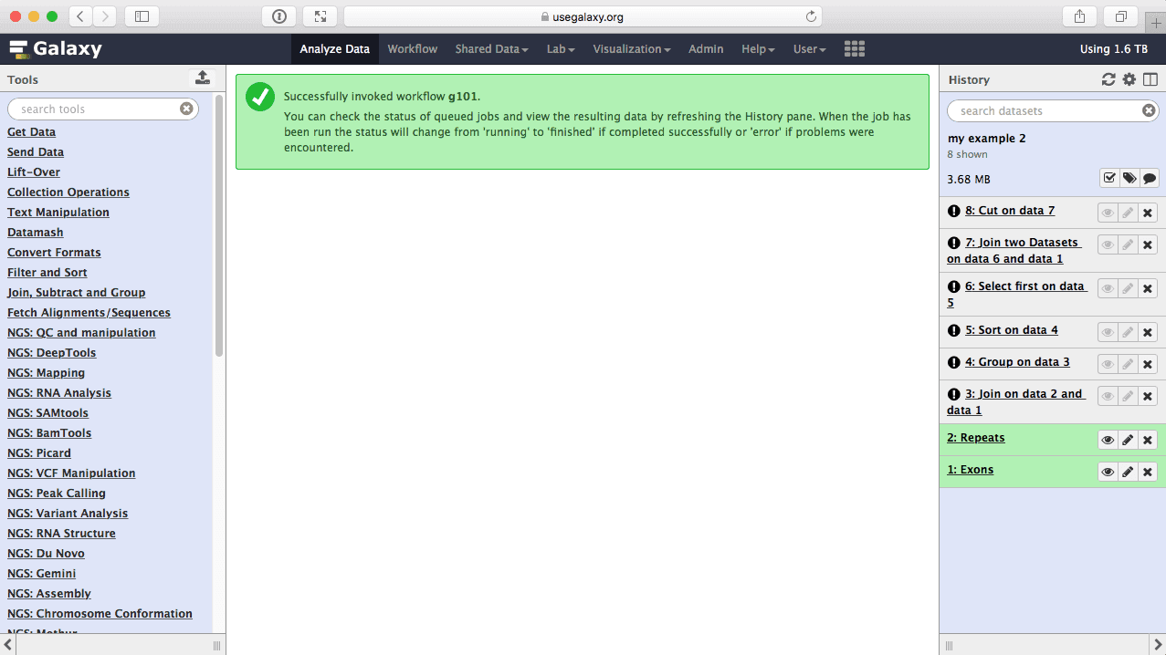figure 46. Workflow execution has started.

Get coffee

As we mentioned above this will take some time, so go get coffee. At last you will see this:

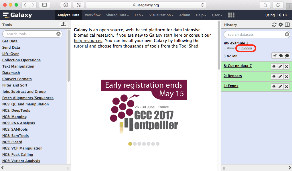Figure 47. The result of running the workflow. Only the final dataset is shown because the intermediate datasets are hidden (see Fig. 33). They can be "unhidden" by clicking on "hidden" link immediate below history name (highlighted in red).

We did not fake this:

The two histories and the workflow described in this page are accessible directly from this page below:

• History my example
• History my example 2
• Workflow g101

From there you can import histories and workflows to make them your own. For example, to import my example history simply click this link and select Import history link:

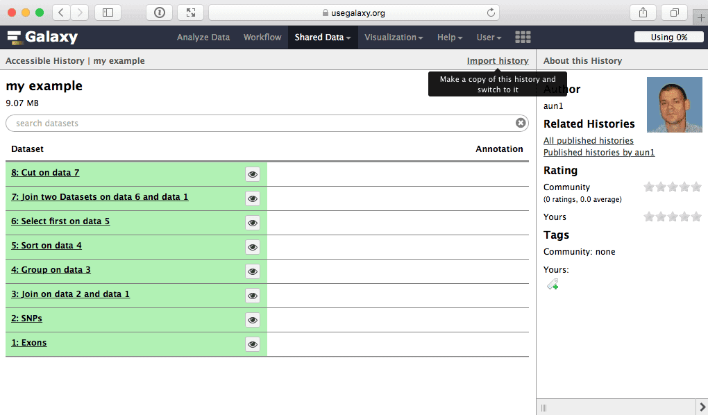|Figure 48. To import a history simply click "Import history" link.

If things don't work...

• ...create an issue by clicking "New issue" button here
• ...complain. Use Galaxy's support forum to do this.